bluemath_tk.datamining package

Submodules

bluemath_tk.datamining.kma module

class bluemath_tk.datamining.kma.KMA(num_clusters: int, seed: int = None)[source]

Bases: BaseClustering

K-Means Algorithm (KMA) class.

This class performs the K-Means algorithm on a given dataframe.

num_clusters

The number of clusters to use in the K-Means algorithm.

Type:: int

seed

The random seed to use as initial datapoint.

Type:: int

data_variables

A list with all data variables.

Type:: List[str]

directional_variables

A list with directional variables.

Type:: List[str]

fitting_variables

A list with fitting variables.

Type:: List[str]

custom_scale_factor

A dictionary of custom scale factors.

Type:: dict

scale_factor

A dictionary of scale factors (after normalizing the data).

Type:: dict

centroids

The selected centroids.

Type:: pd.DataFrame

normalized_centroids

The selected normalized centroids.

Type:: pd.DataFrame

centroid_real_indices

The real indices of the selected centroids.

Type:: np.array

is_fitted

A flag indicating whether the model is fitted or not.

Type:: bool

Examples

import numpy as np
import pandas as pd
from bluemath_tk.datamining.kma import KMA

data = pd.DataFrame(
    {
        "Hs": np.random.rand(1000) * 7,
        "Tp": np.random.rand(1000) * 20,
        "Dir": np.random.rand(1000) * 360
    }
)
kma = KMA(num_clusters=5)
nearest_centroids_idxs, nearest_centroids_df = kma.fit_predict(
    data=data,
    directional_variables=["Dir"],
)

kma.plot_selected_centroids(plot_text=True)

(<Figure size 640x480 with 10 Axes>,
 array([[<Axes: xlabel='Tp', ylabel='Hs'>, <Axes: >, <Axes: >, <Axes: >],
        [<Axes: >, <Axes: xlabel='Dir', ylabel='Tp'>, <Axes: >, <Axes: >],
        [<Axes: >, <Axes: >, <Axes: xlabel='Dir_u', ylabel='Dir'>,
         <Axes: >],
        [<Axes: >, <Axes: >, <Axes: >,
         <Axes: xlabel='Dir_v', ylabel='Dir_u'>]], dtype=object))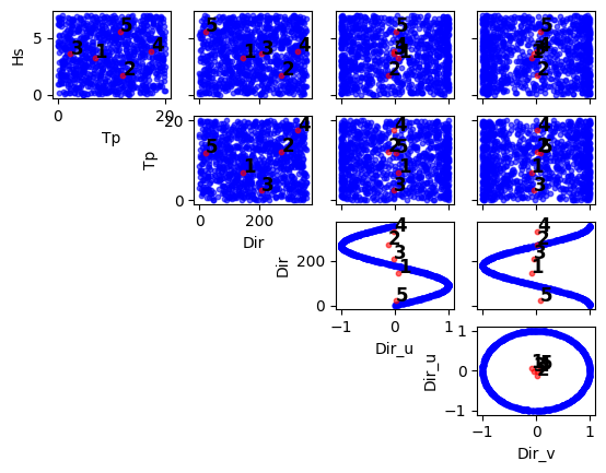

static add_regression_guided(data: DataFrame, vars: List[str], alpha: List[float]) → DataFrame[source]

Calculate regression-guided variables.

Parameters:

data (pd.DataFrame) – The data to fit the K-Means algorithm.
vars (List[str]) – The variables to use for regression-guided clustering.
alpha (List[float]) – The alpha values to use for regression-guided clustering.

Returns:

The data with the regression-guided variables.

Return type:

pd.DataFrame

property data: DataFrame: Returns the original data used for clustering.

property data_to_fit: DataFrame: Returns the data used for fitting the K-Means algorithm.

fit(data: DataFrame, directional_variables: List[str] = [], custom_scale_factor: dict = {}, min_number_of_points: int = None, max_number_of_iterations: int = 10, normalize_data: bool = False, regression_guided: Dict[str, List] = {}) → None[source]

Fit the K-Means algorithm to the provided data.

TODO: Add option to force KMA initialization with MDA centroids.

Parameters:

data (pd.DataFrame) – The input data to be used for the KMA algorithm.
directional_variables (List[str], optional) – A list of directional variables that will be transformed to u and v components. Then, to use custom_scale_factor, you must specify the variables names with the u and v suffixes. Example: directional_variables=[“Dir”], custom_scale_factor={“Dir_u”: [0, 1], “Dir_v”: [0, 1]}. Default is [].
custom_scale_factor (dict, optional) – A dictionary specifying custom scale factors for normalization. If normalize_data is True, this will be used to normalize the data. Example: {“Hs”: [0, 10], “Tp”: [0, 10]}. Default is {}.
min_number_of_points (int, optional) – The minimum number of points to consider a cluster. Default is None.
max_number_of_iterations (int, optional) – The maximum number of iterations for the K-Means algorithm. This is used when min_number_of_points is not None. Default is 10.
normalize_data (bool, optional) – A flag to normalize the data. If True, the data will be normalized using the custom_scale_factor. Default is False.
regression_guided (dict, optional) – A dictionary specifying regression-guided clustering variables and relative weights. Example: {“vars”: [“Fe”], “alpha”: [0.6]}. Default is {}.

fit_predict(data: DataFrame, directional_variables: List[str] = [], custom_scale_factor: dict = {}, min_number_of_points: int = None, max_number_of_iterations: int = 10, normalize_data: bool = False, regression_guided: Dict[str, List] = {}) → Tuple[DataFrame, DataFrame][source]

Fit the K-Means algorithm to the provided data and predict the nearest centroid for each data point.

Parameters:

data (pd.DataFrame) – The input data to be used for the KMA algorithm.
directional_variables (List[str], optional) – A list of directional variables that will be transformed to u and v components. Then, to use custom_scale_factor, you must specify the variables names with the u and v suffixes. Example: directional_variables=[“Dir”], custom_scale_factor={“Dir_u”: [0, 1], “Dir_v”: [0, 1]}. Default is [].
custom_scale_factor (dict, optional) – A dictionary specifying custom scale factors for normalization. If normalize_data is True, this will be used to normalize the data. Example: {“Hs”: [0, 10], “Tp”: [0, 10]}. Default is {}.
min_number_of_points (int, optional) – The minimum number of points to consider a cluster. Default is None.
max_number_of_iterations (int, optional) – The maximum number of iterations for the K-Means algorithm. This is used when min_number_of_points is not None. Default is 10.
normalize_data (bool, optional) – A flag to normalize the data. If True, the data will be normalized using the custom_scale_factor. Default is False.
regression_guided (dict, optional) – A dictionary specifying regression-guided clustering variables and relative weights. Example: {“vars”: [“Fe”], “alpha”: [0.6]}. Default is {}.

Returns:

A tuple containing the nearest centroid index for each data point, and the nearest centroids.

Return type:

Tuple[pd.DataFrame, pd.DataFrame]

property kma: KMeans

property normalized_data: DataFrame: Returns the normalized data used for clustering.

predict(data: DataFrame) → Tuple[DataFrame, DataFrame][source]

Predict the nearest centroid for the provided data.

Parameters:: data (pd.DataFrame) – The input data to be used for the prediction.
Returns:: A tuple containing the nearest centroid index for each data point, and the nearest centroids.
Return type:: Tuple[pd.DataFrame, pd.DataFrame]

exception bluemath_tk.datamining.kma.KMAError(message: str = 'KMA error occurred.')[source]

Bases: Exception

Custom exception for KMA class.

bluemath_tk.datamining.lhs module

class bluemath_tk.datamining.lhs.LHS(num_dimensions: int, seed: int = 1)[source]

Bases: BaseSampling

Latin Hypercube Sampling (LHS) class.

This class performs the LHS algorithm for some input data.

num_dimensions

The number of dimensions to use in the LHS algorithm.

Type:: int

seed

The random seed to use.

Type:: int

lhs

The Latin Hypercube object.

Type:: qdc.LatinHypercube

data

The LHS samples dataframe.

Type:: pd.DataFrame

generate(dimensions_names, lower_bounds, upper_bounds, num_samples)[source]: Generate LHS samples.

Notes

This class is designed to perform the LHS algorithm.

Examples

>>> from bluemath_tk.datamining.lhs import LHS
>>> dimensions_names = ['CM', 'SS', 'Qb']
>>> lower_bounds = [0.5, -0.2, 1]
>>> upper_bounds = [5.3, 1.5, 200]
>>> lhs = LHS(num_dimensions=3, seed=0)
>>> lhs_sampled_df = lhs.generate(
...     dimensions_names=dimensions_names,
...     lower_bounds=lower_bounds,
...     upper_bounds=upper_bounds,
...     num_samples=100,
... )

property data: DataFrame

generate(dimensions_names: List[str], lower_bounds: List[float], upper_bounds: List[float], num_samples: int) → DataFrame[source]

Generate LHS samples.

Parameters:

dimensions_names (List[str]) – The names of the dimensions.
lower_bounds (List[float]) – The lower bounds of the dimensions.
upper_bounds (List[float]) – The upper bounds of the dimensions.
num_samples (int) – The number of samples to generate. Must be greater than 0.

Returns:

self.data – The LHS samples.

Return type:

pd.DataFrame

property lhs: LatinHypercube

exception bluemath_tk.datamining.lhs.LHSError(message: str = 'LHS error occurred.')[source]

Bases: Exception

Custom exception for LHS class.

bluemath_tk.datamining.mda module

class bluemath_tk.datamining.mda.MDA(num_centers: int)[source]

Bases: BaseClustering

Maximum Dissimilarity Algorithm (MDA) class.

This class performs the MDA algorithm on a given dataframe.

num_centers

The number of centers to use in the MDA algorithm.

Type:: int

data_variables

A list with all data variables.

Type:: List[str]

directional_variables

A list with directional variables.

Type:: List[str]

fitting_variables

A list with fitting variables.

Type:: List[str]

custom_scale_factor

A dictionary of custom scale factors.

Type:: dict

scale_factor

A dictionary of scale factors (after normalizing the data).

Type:: dict

centroids

The selected centroids.

Type:: pd.DataFrame

normalized_centroids

The selected normalized centroids.

Type:: pd.DataFrame

centroid_iterative_indices

A list of iterative indices of the centroids.

Type:: List[int]

centroid_real_indices

The real indices of the selected centroids.

Type:: List[int]

is_fitted

A flag indicating whether the model is fitted or not.

Type:: bool

Examples

import numpy as np
import pandas as pd
from bluemath_tk.datamining.mda import MDA

data = pd.DataFrame(
    {
        "Hs": np.random.rand(1000) * 7,
        "Tp": np.random.rand(1000) * 20,
        "Dir": np.random.rand(1000) * 360
    }
)
mda = MDA(num_centers=5)
nearest_centroids_idxs, nearest_centroids_df = mda.fit_predict(
    data=data,
    directional_variables=["Dir"],
)

mda.plot_selected_centroids(plot_text=True)

(<Figure size 640x480 with 10 Axes>,
 array([[<Axes: xlabel='Tp', ylabel='Hs'>, <Axes: >, <Axes: >, <Axes: >],
        [<Axes: >, <Axes: xlabel='Dir', ylabel='Tp'>, <Axes: >, <Axes: >],
        [<Axes: >, <Axes: >, <Axes: xlabel='Dir_u', ylabel='Dir'>,
         <Axes: >],
        [<Axes: >, <Axes: >, <Axes: >,
         <Axes: xlabel='Dir_v', ylabel='Dir_u'>]], dtype=object))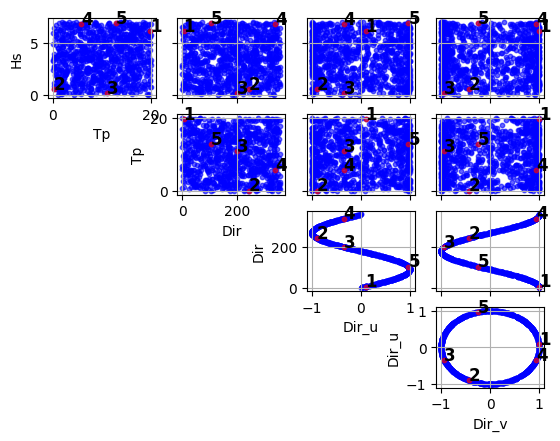

property data: DataFrame: Returns the original data used for clustering.

property data_to_fit: DataFrame: Returns the data used for fitting the K-Means algorithm.

fit(data: DataFrame, directional_variables: List[str] = [], custom_scale_factor: dict = {}, first_centroid_seed: int = None, normalize_data: bool = False) → None[source]

Fit the Maximum Dissimilarity Algorithm (MDA) to the provided data.

This method initializes centroids for the MDA algorithm using the provided dataframe, directional variables, and custom scale factor. It normalizes the data, iteratively selects centroids based on maximum dissimilarity, and denormalizes the centroids before returning them.

Parameters:

data (pd.DataFrame) – The input data to be used for the MDA algorithm.
directional_variables (List[str], optional) – A list of directional variables that will be transformed to u and v components. Then, to use custom_scale_factor, you must specify the variables names with the u and v suffixes. Example: directional_variables=[“Dir”], custom_scale_factor={“Dir_u”: [0, 1], “Dir_v”: [0, 1]}. Default is [].
custom_scale_factor (dict, optional) – A dictionary specifying custom scale factors for normalization. If normalize_data is True, this will be used to normalize the data. Example: {“Hs”: [0, 10], “Tp”: [0, 10]}. Default is {}.
first_centroid_seed (int, optional) – The index of the first centroid to use in the MDA algorithm. Default is None.
normalize_data (bool, optional) – A flag to normalize the data. If True, the data will be normalized using the custom_scale_factor. Default is False.

Notes

When first_centroid_seed is not provided, max value centroid is used.

fit_predict(data: DataFrame, directional_variables: List[str] = [], custom_scale_factor: dict = {}, first_centroid_seed: int = None, normalize_data: bool = False) → Tuple[ndarray, DataFrame][source]

Fits the MDA model to the data and predicts the nearest centroids.

Parameters:

data (pd.DataFrame) – The input data to be used for the MDA algorithm.
directional_variables (List[str], optional) – A list of directional variables that will be transformed to u and v components. Then, to use custom_scale_factor, you must specify the variables names with the u and v suffixes. Example: directional_variables=[“Dir”], custom_scale_factor={“Dir_u”: [0, 1], “Dir_v”: [0, 1]}. Default is [].
custom_scale_factor (dict, optional) – A dictionary specifying custom scale factors for normalization. If normalize_data is True, this will be used to normalize the data. Example: {“Hs”: [0, 10], “Tp”: [0, 10]}. Default is {}.
first_centroid_seed (int, optional) – The index of the first centroid to use in the MDA algorithm. Default is None.
normalize_data (bool, optional) – A flag to normalize the data. If True, the data will be normalized using the custom_scale_factor. Default is False.

Returns:

A tuple containing the nearest centroid index for each data point and the nearest centroids.

Return type:

Tuple[np.ndarray, pd.DataFrame]

property normalized_data: DataFrame: Returns the normalized data used for clustering.

predict(data: DataFrame) → Tuple[ndarray, DataFrame][source]

Predict the nearest centroid for the provided data.

Parameters:: data (pd.DataFrame) – The input data to be used for the prediction.
Returns:: A tuple containing the nearest centroid index for each data point and the nearest centroids.
Return type:: Tuple[np.ndarray, pd.DataFrame]

exception bluemath_tk.datamining.mda.MDAError(message: str = 'MDA error occurred.')[source]

Bases: Exception

Custom exception for MDA class.

bluemath_tk.datamining.mda.calculate_normalized_squared_distance(data_array: ndarray | DataFrame, array_to_compare: ndarray | DataFrame, directional_indices: List[int] = None, weights: List[float] = None) → ndarray[source]

Calculate the normalized squared distance between the data_array and the array_to_compare. ALERT: directional_indices will be deprecated in the future.

Parameters:

data_array (Union[np.ndarray, pd.DataFrame]) – The data array to compare. Dimensions: (1, n_features).
array_to_compare (Union[np.ndarray, pd.DataFrame]) – The array to compare against. Dimensions: (n_samples, n_features).
directional_indices (List[int], optional) – List of column indices that contain directional data. For these columns, the minimum circular distance will be used. Default is None.
weights (List[float], optional) – List of weights to apply to each column’s distance. Must have the same length as the number of columns. Default is None (equal weights).

Returns:

An array of normalized squared distance between the two arrays. Dimensions: (n_samples, 1).

Return type:

np.ndarray

Raises:

ValueError – If the arrays have different numbers of columns. If weights are provided but length doesn’t match number of columns.

Examples

>>> calculate_normalized_squared_distance(
...     data_array=np.array([[1, 2, 3]]),
...     array_to_compare=np.array([[1, 2, 3], [4, 5, 6]]),
... )
[0.0, 27.0]

Notes

IMPORTANT: Data is assumed to be normalized before calling this function.
For directional variables, the function calculates the minimum circular distance. Assuming data is between 0 and 1 (normalized).
The function calculates weighted squared differences for each row.
If DataFrames are provided, they will be converted to numpy arrays.

bluemath_tk.datamining.mda.find_nearest_indices(query_points: ndarray | DataFrame, reference_points: ndarray | DataFrame, directional_indices: List[int] = None, weights: List[float] = None) → ndarray[source]

Find the indices of nearest points in reference_points for each point in query_points.

Parameters:

query_points (Union[np.ndarray, pd.DataFrame]) – The points to find nearest neighbors for.
reference_points (Union[np.ndarray, pd.DataFrame]) – The set of points to search in.
directional_indices (List[int], optional) – List of column indices that contain directional data. For these columns, the minimum circular distance will be used. Default is None.
weights (List[float], optional) – List of weights to apply to each column’s distance. Must have the same length as the number of columns. Default is None (equal weights).

Returns:

An array containing the index of the nearest reference point for each query point.

Return type:

np.ndarray

Examples

>>> # Finding nearest centroids for data points
>>> data = np.random.rand(100, 3)  # 100 points with 3 features
>>> centroids = np.random.rand(5, 3)  # 5 centroids
>>> nearest_centroid_indices = find_nearest_indices(data, centroids)

bluemath_tk.datamining.pca module

class bluemath_tk.datamining.pca.PCA(n_components: int | float = 0.98, is_incremental: bool = False, debug: bool = False)[source]

Bases: BaseReduction

Principal Component Analysis (PCA) class.

n_components

The number of components or the explained variance ratio.

Type:: Union[int, float]

is_incremental

Indicates whether Incremental PCA is used.

Type:: bool

is_fitted

Indicates whether the PCA model has been fitted.

Type:: bool

scaler

The scaler used for standardizing the data, in case the data is standarized.

Type:: StandardScaler

vars_to_stack

The list of variables to stack.

Type:: List[str]

window_stacked_vars

The list of variables with windows.

Type:: List[str]

coords_to_stack

The list of coordinates to stack.

Type:: List[str]

coords_values

The values of the data coordinates used in fitting.

Type:: dict

pca_dim_for_rows

The dimension for rows in PCA.

Type:: str

windows_in_pca_dim_for_rows

The windows in PCA dimension for rows.

Type:: dict

value_to_replace_nans

The values to replace NaNs in the dataset.

Type:: dict

nan_threshold_to_drop

The threshold percentage to drop NaNs for each variable.

Type:: dict

num_cols_for_vars

The number of columns for variables.

Type:: int

pcs

The Principal Components (PCs).

Type:: xr.Dataset

Examples

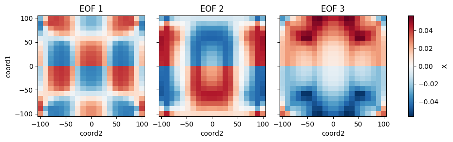
from bluemath_tk.core.data.sample_data import get_2d_dataset
from bluemath_tk.datamining.pca import PCA

ds = get_2d_dataset()

pca = PCA(
    n_components=5,
    is_incremental=False,
    debug=True,
)
pca.fit(
    data=ds,
    vars_to_stack=["X", "Y"],
    coords_to_stack=["coord1", "coord2"],
    pca_dim_for_rows="coord3",
    windows_in_pca_dim_for_rows={"X": [1, 2, 3]},
    value_to_replace_nans={"X": 0.0},
    nan_threshold_to_drop={"X": 0.95},
)
pcs = pca.transform(
    data=ds,
)
reconstructed_ds = pca.inverse_transform(PCs=pcs)
eofs = pca.eofs
explained_variance = pca.explained_variance
explained_variance_ratio = pca.explained_variance_ratio
cumulative_explained_variance_ratio = pca.cumulative_explained_variance_ratio

# Save the full class in a pickle file
pca.save_model("pca_model.pkl")

# Plot the calculated EOFs
pca.plot_eofs(vars_to_plot=["X", "Y"], num_eofs=3)

        -------------------------------------------------------------------
        | Initializing PCA reduction model with the following parameters:
        |    - n_components: 5
        |    - is_incremental: False
        | For more information, please refer to the documentation.
        -------------------------------------------------------------------
        

References

[1] https://scikit-learn.org/stable/modules/generated/sklearn.decomposition.PCA.html

[2] https://scikit-learn.org/stable/modules/generated/sklearn.decomposition.IncrementalPCA.html

[3] https://www.sciencedirect.com/science/article/abs/pii/S0378383911000676

property cumulative_explained_variance_ratio: ndarray: Return the cumulative explained variance ratio of the PCA model.

property data: Dataset: Returns the raw data used for PCA.

property eofs: Dataset: Return the Empirical Orthogonal Functions (EOFs).

property explained_variance: ndarray: Return the explained variance of the PCA model.

property explained_variance_ratio: ndarray: Return the explained variance ratio of the PCA model.

fit(data: Dataset, vars_to_stack: List[str], coords_to_stack: List[str], pca_dim_for_rows: str, windows_in_pca_dim_for_rows: dict = {}, value_to_replace_nans: dict = {}, nan_threshold_to_drop: dict = {}, scale_data: bool = True) → None[source]

Fit PCA model to data.

Parameters:

data (xr.Dataset) – The data to fit the PCA model.
vars_to_stack (list of str) – The variables to stack.
coords_to_stack (list of str) – The coordinates to stack.
pca_dim_for_rows (str) – The PCA dimension to maintain in rows (usually the time).
windows_in_pca_dim_for_rows (dict, optional) – The window steps to roll the pca_dim_for_rows for each variable. Default is {}.
value_to_replace_nans (dict, optional) – The value to replace NaNs for each variable. Default is {}.
nan_threshold_to_drop (dict, optional) – The threshold percentage to drop NaNs for each variable. By default, variables with less than 90% of valid values are dropped, which corresponds to {‘ALL_vars’: 0.9}. To for example use all available data for variable ‘wind’, you must provide nan_threshold_to_drop: {‘wind’: 1e-9}. Default is {}.
scale_data (bool, optional) – If True, scale the data. Default is True.

Notes

For both value_to_replace_nans and nan_threshold_to_drop, the keys are the variables, and the suffixes for the windows are considered. Example: if you have variable “X”, and apply windows [1, 2, 3], you can use “X_1”, “X_2”, “X_3”. Nevertheless, you can also use the original variable name “X” to apply the same value for all windows.

fit_transform(data: Dataset, vars_to_stack: List[str], coords_to_stack: List[str], pca_dim_for_rows: str, windows_in_pca_dim_for_rows: dict = {}, value_to_replace_nans: dict = {}, nan_threshold_to_drop: dict = {}, scale_data: bool = True) → Dataset[source]

Fit and transform data using PCA model.

Parameters:

data (xr.Dataset) – The data to fit the PCA model.
vars_to_stack (list of str) – The variables to stack.
coords_to_stack (list of str) – The coordinates to stack.
pca_dim_for_rows (str) – The PCA dimension to maintain in rows (usually the time).
windows_in_pca_dim_for_rows (dict, optional) – The window steps to roll the pca_dim_for_rows for each variable. Default is {}.
value_to_replace_nans (dict, optional) – The value to replace NaNs for each variable. Default is {}.
nan_threshold_to_drop (dict, optional) – The threshold percentage to drop NaNs for each variable. By default, variables with less than 90% of valid values are dropped, which corresponds to {‘ALL_vars’: 0.9}. To for example use all available data for variable ‘wind’, you must provide nan_threshold_to_drop: {‘wind’: 1e-9}. Default is {}.
scale_data (bool, optional) – If True, scale the data. Default is True.

Returns:

The transformed data representing the Principal Components (PCs).

Return type:

xr.Dataset

Notes

For both value_to_replace_nans and nan_threshold_to_drop, the keys are the variables, and the suffixes for the windows are considered. Example: if you have variable “X”, and apply windows [1, 2, 3], you can use “X_1”, “X_2”, “X_3”. Nevertheless, you can also use the original variable name “X” to apply the same value for all windows.

inverse_transform(PCs: DataArray | Dataset) → Dataset[source]

Inverse transform data using the fitted PCA model.

Parameters:: PCs (Union[xr.DataArray, xr.Dataset]) – The data to inverse transform. It should be the Principal Components (PCs).
Returns:: The inverse transformed data.
Return type:: xr.Dataset

property pca: PCA | IncrementalPCA: Returns the PCA or IncrementalPCA instance used for dimensionality reduction.

property pcs_df: DataFrame: Returns the principal components as a DataFrame.

plot_eofs(vars_to_plot: List[str], num_eofs: int, destandarize: bool = False, map_center: tuple = None) → None[source]

Plot the Empirical Orthogonal Functions (EOFs).

Parameters:

vars_to_plot (List[str]) – The variables to plot.
num_eofs (int) – The number of EOFs to plot.
destandarize (bool, optional) – If True, destandarize the EOFs. Default is False.
map_center (tuple, optional) – The center of the map. Default is None. First value is the longitude (-180, 180), and the second value is the latitude (-90, 90).

plot_pcs(num_pcs: int, pcs: Dataset = None) → None[source]

Plot the Principal Components (PCs).

Parameters:

num_pcs (int) – The number of Principal Components (PCs) to plot.
pcs (xr.Dataset, optional) – The Principal Components (PCs) to plot.

property stacked_data_matrix: ndarray: Return the stacked data matrix.

property standarized_stacked_data_matrix: ndarray: Return the standarized stacked data matrix.

transform(data: Dataset, after_fitting: bool = False) → Dataset[source]

Transform data using the fitted PCA model.

Parameters:

data (xr.Dataset) – The data to transform.
after_fitting (bool, optional) – If True, use the already processed data. Default is False. This is just used in the fit_transform method!

Returns:

The transformed data.

Return type:

xr.Dataset

property window_processed_data: Dataset: Return the window processed data used for PCA.

exception bluemath_tk.datamining.pca.PCAError(message: str = 'PCA error occurred.')[source]

Bases: Exception

Custom exception for PCA class.

bluemath_tk.datamining.som module

class bluemath_tk.datamining.som.SOM(som_shape: Tuple[int, int], num_dimensions: int, sigma: float = 1, learning_rate: float = 0.5, decay_function: str = 'asymptotic_decay', neighborhood_function: str = 'gaussian', topology: str = 'rectangular', activation_distance: str = 'euclidean', random_seed: int = None, sigma_decay_function: str = 'asymptotic_decay')[source]

Bases: BaseClustering

Self-Organizing Maps (SOM) class.

This class performs the Self-Organizing Map algorithm on a given dataframe.

som_shape

The shape of the SOM.

Type:: Tuple[int, int]

num_dimensions

The number of dimensions of the input data.

Type:: int

data_variables

A list with all data variables.

Type:: List[str]

directional_variables

A list with directional variables.

Type:: List[str]

fitting_variables

A list with fitting variables.

Type:: List[str]

custom_scale_factor

A dictionary of custom scale factors.

Type:: dict

scale_factor

A dictionary of scale factors (after normalizing the data).

Type:: dict

centroids

The selected centroids.

Type:: pd.DataFrame

normalized_centroids

The selected normalized centroids.

Type:: pd.DataFrame

is_fitted

A flag to check if the SOM model is fitted.

Type:: bool

Notes

Check MiniSom documentation for more information:
https://github.com/JustGlowing/minisom

Examples

:: jupyter-execute:

import numpy as np
import pandas as pd
from bluemath_tk.datamining.som import SOM

data = pd.DataFrame(
    {
        "Hs": np.random.rand(1000) * 7,
        "Tp": np.random.rand(1000) * 20,
        "Dir": np.random.rand(1000) * 360
    }
)
som = SOM(som_shape=(3, 3), num_dimensions=4)
nearest_centroids_idxs, nearest_centroids_df = som.fit_predict(
    data=data,
    directional_variables=["Dir"],
)

som.plot_selected_centroids(plot_text=True)

activation_response(data: DataFrame = None) → ndarray[source]: Returns the activation response of the given data.

property data: DataFrame: Returns the original data used for clustering.

property data_to_fit: DataFrame: Returns the data used for fitting the K-Means algorithm.

property distance_map: ndarray: Returns the distance map of the SOM.

fit(data: DataFrame, directional_variables: List[str] = [], custom_scale_factor: dict = {}, num_iteration: int = 1000, normalize_data: bool = False) → None[source]

Fits the SOM model to the provided data.

Parameters:

data (pd.DataFrame) – The input data to be used for the SOM algorithm.
directional_variables (List[str], optional) – A list of directional variables that will be transformed to u and v components. Then, to use custom_scale_factor, you must specify the variables names with the u and v suffixes. Example: directional_variables=[“Dir”], custom_scale_factor={“Dir_u”: [0, 1], “Dir_v”: [0, 1]}. Default is [].
custom_scale_factor (dict, optional) – A dictionary specifying custom scale factors for normalization. If normalize_data is True, this will be used to normalize the data. Example: {“Hs”: [0, 10], “Tp”: [0, 10]}. Default is {}.
num_iteration (int, optional) – The number of iterations for the SOM fitting. Default is 1000.
normalize_data (bool, optional) – A flag to normalize the data. If True, the data will be normalized using the custom_scale_factor. Default is False.

fit_predict(data: DataFrame, directional_variables: List[str] = [], custom_scale_factor: dict = {}, num_iteration: int = 1000, normalize_data: bool = False) → Tuple[ndarray, DataFrame][source]

Fit the SOM algorithm to the provided data and predict the nearest centroid for each data point.

Parameters:

data (pd.DataFrame) – The input data to be used for the SOM algorithm.
directional_variables (List[str], optional) – A list of directional variables that will be transformed to u and v components. Then, to use custom_scale_factor, you must specify the variables names with the u and v suffixes. Example: directional_variables=[“Dir”], custom_scale_factor={“Dir_u”: [0, 1], “Dir_v”: [0, 1]}. Default is [].
custom_scale_factor (dict, optional) – A dictionary specifying custom scale factors for normalization. If normalize_data is True, this will be used to normalize the data. Example: {“Hs”: [0, 10], “Tp”: [0, 10]}. Default is {}.
num_iteration (int, optional) – The number of iterations for the SOM fitting. Default is 1000.
normalize_data (bool, optional) – A flag to normalize the data. If True, the data will be normalized using the custom_scale_factor. Default is False.

Returns:

A tuple containing the winner neurons for each data point and the nearest centroids.

Return type:

Tuple[np.ndarray, pd.DataFrame]

get_centroids_probs_for_labels(data: DataFrame, labels: List[str]) → DataFrame[source]: Returns the labels map of the given data.

property normalized_data: DataFrame: Returns the normalized data used for clustering.

plot_centroids_probs_for_labels(probs_data: DataFrame) → Tuple[figure, axes][source]: Plots the labels map of the given data.

predict(data: DataFrame) → Tuple[ndarray, DataFrame][source]

Predicts the nearest centroid for the provided data.

Parameters:: data (pd.DataFrame) – The input data to be used for the prediction.
Returns:: A tuple with the winner neurons and the centroids of the given data.
Return type:: Tuple[np.ndarray, pd.DataFrame]

property som: MiniSom

exception bluemath_tk.datamining.som.SOMError(message: str = 'SOM error occurred.')[source]

Bases: Exception

Custom exception for SOM class.

Module contents

Project: BlueMath_tk Sub-Module: datamining Author: GeoOcean Research Group, Universidad de Cantabria Repository: https://github.com/GeoOcean/BlueMath_tk.git Status: Under development (Working)

class bluemath_tk.datamining.KMA(num_clusters: int, seed: int = None)[source]

Bases: BaseClustering

K-Means Algorithm (KMA) class.

This class performs the K-Means algorithm on a given dataframe.

num_clusters

The number of clusters to use in the K-Means algorithm.

Type:: int

seed

The random seed to use as initial datapoint.

Type:: int

data_variables

A list with all data variables.

Type:: List[str]

directional_variables

A list with directional variables.

Type:: List[str]

fitting_variables

A list with fitting variables.

Type:: List[str]

custom_scale_factor

A dictionary of custom scale factors.

Type:: dict

scale_factor

A dictionary of scale factors (after normalizing the data).

Type:: dict

centroids

The selected centroids.

Type:: pd.DataFrame

normalized_centroids

The selected normalized centroids.

Type:: pd.DataFrame

centroid_real_indices

The real indices of the selected centroids.

Type:: np.array

is_fitted

A flag indicating whether the model is fitted or not.

Type:: bool

Examples

import numpy as np
import pandas as pd
from bluemath_tk.datamining.kma import KMA

data = pd.DataFrame(
    {
        "Hs": np.random.rand(1000) * 7,
        "Tp": np.random.rand(1000) * 20,
        "Dir": np.random.rand(1000) * 360
    }
)
kma = KMA(num_clusters=5)
nearest_centroids_idxs, nearest_centroids_df = kma.fit_predict(
    data=data,
    directional_variables=["Dir"],
)

kma.plot_selected_centroids(plot_text=True)

(<Figure size 640x480 with 10 Axes>,
 array([[<Axes: xlabel='Tp', ylabel='Hs'>, <Axes: >, <Axes: >, <Axes: >],
        [<Axes: >, <Axes: xlabel='Dir', ylabel='Tp'>, <Axes: >, <Axes: >],
        [<Axes: >, <Axes: >, <Axes: xlabel='Dir_u', ylabel='Dir'>,
         <Axes: >],
        [<Axes: >, <Axes: >, <Axes: >,
         <Axes: xlabel='Dir_v', ylabel='Dir_u'>]], dtype=object))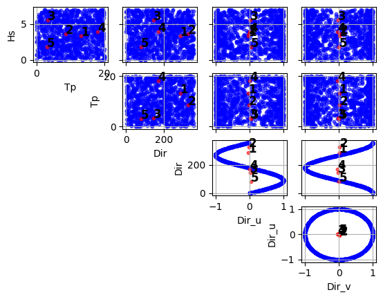

static add_regression_guided(data: DataFrame, vars: List[str], alpha: List[float]) → DataFrame[source]

Calculate regression-guided variables.

Parameters:

data (pd.DataFrame) – The data to fit the K-Means algorithm.
vars (List[str]) – The variables to use for regression-guided clustering.
alpha (List[float]) – The alpha values to use for regression-guided clustering.

Returns:

The data with the regression-guided variables.

Return type:

pd.DataFrame

property data: DataFrame: Returns the original data used for clustering.

property data_to_fit: DataFrame: Returns the data used for fitting the K-Means algorithm.

fit(data: DataFrame, directional_variables: List[str] = [], custom_scale_factor: dict = {}, min_number_of_points: int = None, max_number_of_iterations: int = 10, normalize_data: bool = False, regression_guided: Dict[str, List] = {}) → None[source]

Fit the K-Means algorithm to the provided data.

TODO: Add option to force KMA initialization with MDA centroids.

Parameters:

data (pd.DataFrame) – The input data to be used for the KMA algorithm.
directional_variables (List[str], optional) – A list of directional variables that will be transformed to u and v components. Then, to use custom_scale_factor, you must specify the variables names with the u and v suffixes. Example: directional_variables=[“Dir”], custom_scale_factor={“Dir_u”: [0, 1], “Dir_v”: [0, 1]}. Default is [].
custom_scale_factor (dict, optional) – A dictionary specifying custom scale factors for normalization. If normalize_data is True, this will be used to normalize the data. Example: {“Hs”: [0, 10], “Tp”: [0, 10]}. Default is {}.
min_number_of_points (int, optional) – The minimum number of points to consider a cluster. Default is None.
max_number_of_iterations (int, optional) – The maximum number of iterations for the K-Means algorithm. This is used when min_number_of_points is not None. Default is 10.
normalize_data (bool, optional) – A flag to normalize the data. If True, the data will be normalized using the custom_scale_factor. Default is False.
regression_guided (dict, optional) – A dictionary specifying regression-guided clustering variables and relative weights. Example: {“vars”: [“Fe”], “alpha”: [0.6]}. Default is {}.

fit_predict(data: DataFrame, directional_variables: List[str] = [], custom_scale_factor: dict = {}, min_number_of_points: int = None, max_number_of_iterations: int = 10, normalize_data: bool = False, regression_guided: Dict[str, List] = {}) → Tuple[DataFrame, DataFrame][source]

Fit the K-Means algorithm to the provided data and predict the nearest centroid for each data point.

Parameters:

data (pd.DataFrame) – The input data to be used for the KMA algorithm.
directional_variables (List[str], optional) – A list of directional variables that will be transformed to u and v components. Then, to use custom_scale_factor, you must specify the variables names with the u and v suffixes. Example: directional_variables=[“Dir”], custom_scale_factor={“Dir_u”: [0, 1], “Dir_v”: [0, 1]}. Default is [].
custom_scale_factor (dict, optional) – A dictionary specifying custom scale factors for normalization. If normalize_data is True, this will be used to normalize the data. Example: {“Hs”: [0, 10], “Tp”: [0, 10]}. Default is {}.
min_number_of_points (int, optional) – The minimum number of points to consider a cluster. Default is None.
max_number_of_iterations (int, optional) – The maximum number of iterations for the K-Means algorithm. This is used when min_number_of_points is not None. Default is 10.
normalize_data (bool, optional) – A flag to normalize the data. If True, the data will be normalized using the custom_scale_factor. Default is False.
regression_guided (dict, optional) – A dictionary specifying regression-guided clustering variables and relative weights. Example: {“vars”: [“Fe”], “alpha”: [0.6]}. Default is {}.

Returns:

A tuple containing the nearest centroid index for each data point, and the nearest centroids.

Return type:

Tuple[pd.DataFrame, pd.DataFrame]

property kma: KMeans

property normalized_data: DataFrame: Returns the normalized data used for clustering.

predict(data: DataFrame) → Tuple[DataFrame, DataFrame][source]

Predict the nearest centroid for the provided data.

Parameters:: data (pd.DataFrame) – The input data to be used for the prediction.
Returns:: A tuple containing the nearest centroid index for each data point, and the nearest centroids.
Return type:: Tuple[pd.DataFrame, pd.DataFrame]

class bluemath_tk.datamining.LHS(num_dimensions: int, seed: int = 1)[source]

Bases: BaseSampling

Latin Hypercube Sampling (LHS) class.

This class performs the LHS algorithm for some input data.

num_dimensions

The number of dimensions to use in the LHS algorithm.

Type:: int

seed

The random seed to use.

Type:: int

lhs

The Latin Hypercube object.

Type:: qdc.LatinHypercube

data

The LHS samples dataframe.

Type:: pd.DataFrame

generate(dimensions_names, lower_bounds, upper_bounds, num_samples)[source]: Generate LHS samples.

Notes

This class is designed to perform the LHS algorithm.

Examples

>>> from bluemath_tk.datamining.lhs import LHS
>>> dimensions_names = ['CM', 'SS', 'Qb']
>>> lower_bounds = [0.5, -0.2, 1]
>>> upper_bounds = [5.3, 1.5, 200]
>>> lhs = LHS(num_dimensions=3, seed=0)
>>> lhs_sampled_df = lhs.generate(
...     dimensions_names=dimensions_names,
...     lower_bounds=lower_bounds,
...     upper_bounds=upper_bounds,
...     num_samples=100,
... )

property data: DataFrame

generate(dimensions_names: List[str], lower_bounds: List[float], upper_bounds: List[float], num_samples: int) → DataFrame[source]

Generate LHS samples.

Parameters:

dimensions_names (List[str]) – The names of the dimensions.
lower_bounds (List[float]) – The lower bounds of the dimensions.
upper_bounds (List[float]) – The upper bounds of the dimensions.
num_samples (int) – The number of samples to generate. Must be greater than 0.

Returns:

self.data – The LHS samples.

Return type:

pd.DataFrame

property lhs: LatinHypercube

class bluemath_tk.datamining.MDA(num_centers: int)[source]

Bases: BaseClustering

Maximum Dissimilarity Algorithm (MDA) class.

This class performs the MDA algorithm on a given dataframe.

num_centers

The number of centers to use in the MDA algorithm.

Type:: int

data_variables

A list with all data variables.

Type:: List[str]

directional_variables

A list with directional variables.

Type:: List[str]

fitting_variables

A list with fitting variables.

Type:: List[str]

custom_scale_factor

A dictionary of custom scale factors.

Type:: dict

scale_factor

A dictionary of scale factors (after normalizing the data).

Type:: dict

centroids

The selected centroids.

Type:: pd.DataFrame

normalized_centroids

The selected normalized centroids.

Type:: pd.DataFrame

centroid_iterative_indices

A list of iterative indices of the centroids.

Type:: List[int]

centroid_real_indices

The real indices of the selected centroids.

Type:: List[int]

is_fitted

A flag indicating whether the model is fitted or not.

Type:: bool

Examples

import numpy as np
import pandas as pd
from bluemath_tk.datamining.mda import MDA

data = pd.DataFrame(
    {
        "Hs": np.random.rand(1000) * 7,
        "Tp": np.random.rand(1000) * 20,
        "Dir": np.random.rand(1000) * 360
    }
)
mda = MDA(num_centers=5)
nearest_centroids_idxs, nearest_centroids_df = mda.fit_predict(
    data=data,
    directional_variables=["Dir"],
)

mda.plot_selected_centroids(plot_text=True)

(<Figure size 640x480 with 10 Axes>,
 array([[<Axes: xlabel='Tp', ylabel='Hs'>, <Axes: >, <Axes: >, <Axes: >],
        [<Axes: >, <Axes: xlabel='Dir', ylabel='Tp'>, <Axes: >, <Axes: >],
        [<Axes: >, <Axes: >, <Axes: xlabel='Dir_u', ylabel='Dir'>,
         <Axes: >],
        [<Axes: >, <Axes: >, <Axes: >,
         <Axes: xlabel='Dir_v', ylabel='Dir_u'>]], dtype=object))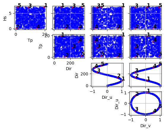

property data: DataFrame: Returns the original data used for clustering.

property data_to_fit: DataFrame: Returns the data used for fitting the K-Means algorithm.

fit(data: DataFrame, directional_variables: List[str] = [], custom_scale_factor: dict = {}, first_centroid_seed: int = None, normalize_data: bool = False) → None[source]

Fit the Maximum Dissimilarity Algorithm (MDA) to the provided data.

This method initializes centroids for the MDA algorithm using the provided dataframe, directional variables, and custom scale factor. It normalizes the data, iteratively selects centroids based on maximum dissimilarity, and denormalizes the centroids before returning them.

Parameters:

data (pd.DataFrame) – The input data to be used for the MDA algorithm.
directional_variables (List[str], optional) – A list of directional variables that will be transformed to u and v components. Then, to use custom_scale_factor, you must specify the variables names with the u and v suffixes. Example: directional_variables=[“Dir”], custom_scale_factor={“Dir_u”: [0, 1], “Dir_v”: [0, 1]}. Default is [].
custom_scale_factor (dict, optional) – A dictionary specifying custom scale factors for normalization. If normalize_data is True, this will be used to normalize the data. Example: {“Hs”: [0, 10], “Tp”: [0, 10]}. Default is {}.
first_centroid_seed (int, optional) – The index of the first centroid to use in the MDA algorithm. Default is None.
normalize_data (bool, optional) – A flag to normalize the data. If True, the data will be normalized using the custom_scale_factor. Default is False.

Notes

When first_centroid_seed is not provided, max value centroid is used.

fit_predict(data: DataFrame, directional_variables: List[str] = [], custom_scale_factor: dict = {}, first_centroid_seed: int = None, normalize_data: bool = False) → Tuple[ndarray, DataFrame][source]

Fits the MDA model to the data and predicts the nearest centroids.

Parameters:

data (pd.DataFrame) – The input data to be used for the MDA algorithm.
directional_variables (List[str], optional) – A list of directional variables that will be transformed to u and v components. Then, to use custom_scale_factor, you must specify the variables names with the u and v suffixes. Example: directional_variables=[“Dir”], custom_scale_factor={“Dir_u”: [0, 1], “Dir_v”: [0, 1]}. Default is [].
custom_scale_factor (dict, optional) – A dictionary specifying custom scale factors for normalization. If normalize_data is True, this will be used to normalize the data. Example: {“Hs”: [0, 10], “Tp”: [0, 10]}. Default is {}.
first_centroid_seed (int, optional) – The index of the first centroid to use in the MDA algorithm. Default is None.
normalize_data (bool, optional) – A flag to normalize the data. If True, the data will be normalized using the custom_scale_factor. Default is False.

Returns:

A tuple containing the nearest centroid index for each data point and the nearest centroids.

Return type:

Tuple[np.ndarray, pd.DataFrame]

property normalized_data: DataFrame: Returns the normalized data used for clustering.

predict(data: DataFrame) → Tuple[ndarray, DataFrame][source]

Predict the nearest centroid for the provided data.

Parameters:: data (pd.DataFrame) – The input data to be used for the prediction.
Returns:: A tuple containing the nearest centroid index for each data point and the nearest centroids.
Return type:: Tuple[np.ndarray, pd.DataFrame]

class bluemath_tk.datamining.PCA(n_components: int | float = 0.98, is_incremental: bool = False, debug: bool = False)[source]

Bases: BaseReduction

Principal Component Analysis (PCA) class.

n_components

The number of components or the explained variance ratio.

Type:: Union[int, float]

is_incremental

Indicates whether Incremental PCA is used.

Type:: bool

is_fitted

Indicates whether the PCA model has been fitted.

Type:: bool

scaler

The scaler used for standardizing the data, in case the data is standarized.

Type:: StandardScaler

vars_to_stack

The list of variables to stack.

Type:: List[str]

window_stacked_vars

The list of variables with windows.

Type:: List[str]

coords_to_stack

The list of coordinates to stack.

Type:: List[str]

coords_values

The values of the data coordinates used in fitting.

Type:: dict

pca_dim_for_rows

The dimension for rows in PCA.

Type:: str

windows_in_pca_dim_for_rows

The windows in PCA dimension for rows.

Type:: dict

value_to_replace_nans

The values to replace NaNs in the dataset.

Type:: dict

nan_threshold_to_drop

The threshold percentage to drop NaNs for each variable.

Type:: dict

num_cols_for_vars

The number of columns for variables.

Type:: int

pcs

The Principal Components (PCs).

Type:: xr.Dataset

Examples

from bluemath_tk.core.data.sample_data import get_2d_dataset
from bluemath_tk.datamining.pca import PCA

ds = get_2d_dataset()

pca = PCA(
    n_components=5,
    is_incremental=False,
    debug=True,
)
pca.fit(
    data=ds,
    vars_to_stack=["X", "Y"],
    coords_to_stack=["coord1", "coord2"],
    pca_dim_for_rows="coord3",
    windows_in_pca_dim_for_rows={"X": [1, 2, 3]},
    value_to_replace_nans={"X": 0.0},
    nan_threshold_to_drop={"X": 0.95},
)
pcs = pca.transform(
    data=ds,
)
reconstructed_ds = pca.inverse_transform(PCs=pcs)
eofs = pca.eofs
explained_variance = pca.explained_variance
explained_variance_ratio = pca.explained_variance_ratio
cumulative_explained_variance_ratio = pca.cumulative_explained_variance_ratio

# Save the full class in a pickle file
pca.save_model("pca_model.pkl")

# Plot the calculated EOFs
pca.plot_eofs(vars_to_plot=["X", "Y"], num_eofs=3)

        -------------------------------------------------------------------
        | Initializing PCA reduction model with the following parameters:
        |    - n_components: 5
        |    - is_incremental: False
        | For more information, please refer to the documentation.
        -------------------------------------------------------------------
        

References

[1] https://scikit-learn.org/stable/modules/generated/sklearn.decomposition.PCA.html

[2] https://scikit-learn.org/stable/modules/generated/sklearn.decomposition.IncrementalPCA.html

[3] https://www.sciencedirect.com/science/article/abs/pii/S0378383911000676

property cumulative_explained_variance_ratio: ndarray: Return the cumulative explained variance ratio of the PCA model.

property data: Dataset: Returns the raw data used for PCA.

property eofs: Dataset: Return the Empirical Orthogonal Functions (EOFs).

property explained_variance: ndarray: Return the explained variance of the PCA model.

property explained_variance_ratio: ndarray: Return the explained variance ratio of the PCA model.

fit(data: Dataset, vars_to_stack: List[str], coords_to_stack: List[str], pca_dim_for_rows: str, windows_in_pca_dim_for_rows: dict = {}, value_to_replace_nans: dict = {}, nan_threshold_to_drop: dict = {}, scale_data: bool = True) → None[source]

Fit PCA model to data.

Parameters:

data (xr.Dataset) – The data to fit the PCA model.
vars_to_stack (list of str) – The variables to stack.
coords_to_stack (list of str) – The coordinates to stack.
pca_dim_for_rows (str) – The PCA dimension to maintain in rows (usually the time).
windows_in_pca_dim_for_rows (dict, optional) – The window steps to roll the pca_dim_for_rows for each variable. Default is {}.
value_to_replace_nans (dict, optional) – The value to replace NaNs for each variable. Default is {}.
nan_threshold_to_drop (dict, optional) – The threshold percentage to drop NaNs for each variable. By default, variables with less than 90% of valid values are dropped, which corresponds to {‘ALL_vars’: 0.9}. To for example use all available data for variable ‘wind’, you must provide nan_threshold_to_drop: {‘wind’: 1e-9}. Default is {}.
scale_data (bool, optional) – If True, scale the data. Default is True.

Notes

For both value_to_replace_nans and nan_threshold_to_drop, the keys are the variables, and the suffixes for the windows are considered. Example: if you have variable “X”, and apply windows [1, 2, 3], you can use “X_1”, “X_2”, “X_3”. Nevertheless, you can also use the original variable name “X” to apply the same value for all windows.

fit_transform(data: Dataset, vars_to_stack: List[str], coords_to_stack: List[str], pca_dim_for_rows: str, windows_in_pca_dim_for_rows: dict = {}, value_to_replace_nans: dict = {}, nan_threshold_to_drop: dict = {}, scale_data: bool = True) → Dataset[source]

Fit and transform data using PCA model.

Parameters:

data (xr.Dataset) – The data to fit the PCA model.
vars_to_stack (list of str) – The variables to stack.
coords_to_stack (list of str) – The coordinates to stack.
pca_dim_for_rows (str) – The PCA dimension to maintain in rows (usually the time).
windows_in_pca_dim_for_rows (dict, optional) – The window steps to roll the pca_dim_for_rows for each variable. Default is {}.
value_to_replace_nans (dict, optional) – The value to replace NaNs for each variable. Default is {}.
nan_threshold_to_drop (dict, optional) – The threshold percentage to drop NaNs for each variable. By default, variables with less than 90% of valid values are dropped, which corresponds to {‘ALL_vars’: 0.9}. To for example use all available data for variable ‘wind’, you must provide nan_threshold_to_drop: {‘wind’: 1e-9}. Default is {}.
scale_data (bool, optional) – If True, scale the data. Default is True.

Returns:

The transformed data representing the Principal Components (PCs).

Return type:

xr.Dataset

Notes

For both value_to_replace_nans and nan_threshold_to_drop, the keys are the variables, and the suffixes for the windows are considered. Example: if you have variable “X”, and apply windows [1, 2, 3], you can use “X_1”, “X_2”, “X_3”. Nevertheless, you can also use the original variable name “X” to apply the same value for all windows.

inverse_transform(PCs: DataArray | Dataset) → Dataset[source]

Inverse transform data using the fitted PCA model.

Parameters:: PCs (Union[xr.DataArray, xr.Dataset]) – The data to inverse transform. It should be the Principal Components (PCs).
Returns:: The inverse transformed data.
Return type:: xr.Dataset

property pca: PCA | IncrementalPCA: Returns the PCA or IncrementalPCA instance used for dimensionality reduction.

property pcs_df: DataFrame: Returns the principal components as a DataFrame.

plot_eofs(vars_to_plot: List[str], num_eofs: int, destandarize: bool = False, map_center: tuple = None) → None[source]

Plot the Empirical Orthogonal Functions (EOFs).

Parameters:

vars_to_plot (List[str]) – The variables to plot.
num_eofs (int) – The number of EOFs to plot.
destandarize (bool, optional) – If True, destandarize the EOFs. Default is False.
map_center (tuple, optional) – The center of the map. Default is None. First value is the longitude (-180, 180), and the second value is the latitude (-90, 90).

plot_pcs(num_pcs: int, pcs: Dataset = None) → None[source]

Plot the Principal Components (PCs).

Parameters:

num_pcs (int) – The number of Principal Components (PCs) to plot.
pcs (xr.Dataset, optional) – The Principal Components (PCs) to plot.

property stacked_data_matrix: ndarray: Return the stacked data matrix.

property standarized_stacked_data_matrix: ndarray: Return the standarized stacked data matrix.

transform(data: Dataset, after_fitting: bool = False) → Dataset[source]

Transform data using the fitted PCA model.

Parameters:

data (xr.Dataset) – The data to transform.
after_fitting (bool, optional) – If True, use the already processed data. Default is False. This is just used in the fit_transform method!

Returns:

The transformed data.

Return type:

xr.Dataset

property window_processed_data: Dataset: Return the window processed data used for PCA.

class bluemath_tk.datamining.SOM(som_shape: Tuple[int, int], num_dimensions: int, sigma: float = 1, learning_rate: float = 0.5, decay_function: str = 'asymptotic_decay', neighborhood_function: str = 'gaussian', topology: str = 'rectangular', activation_distance: str = 'euclidean', random_seed: int = None, sigma_decay_function: str = 'asymptotic_decay')[source]

Bases: BaseClustering

Self-Organizing Maps (SOM) class.

This class performs the Self-Organizing Map algorithm on a given dataframe.

som_shape

The shape of the SOM.

Type:: Tuple[int, int]

num_dimensions

The number of dimensions of the input data.

Type:: int

data_variables

A list with all data variables.

Type:: List[str]

directional_variables

A list with directional variables.

Type:: List[str]

fitting_variables

A list with fitting variables.

Type:: List[str]

custom_scale_factor

A dictionary of custom scale factors.

Type:: dict

scale_factor

A dictionary of scale factors (after normalizing the data).

Type:: dict

centroids

The selected centroids.

Type:: pd.DataFrame

normalized_centroids

The selected normalized centroids.

Type:: pd.DataFrame

is_fitted

A flag to check if the SOM model is fitted.

Type:: bool

Notes

Check MiniSom documentation for more information:
https://github.com/JustGlowing/minisom

Examples

:: jupyter-execute:

import numpy as np
import pandas as pd
from bluemath_tk.datamining.som import SOM

data = pd.DataFrame(
    {
        "Hs": np.random.rand(1000) * 7,
        "Tp": np.random.rand(1000) * 20,
        "Dir": np.random.rand(1000) * 360
    }
)
som = SOM(som_shape=(3, 3), num_dimensions=4)
nearest_centroids_idxs, nearest_centroids_df = som.fit_predict(
    data=data,
    directional_variables=["Dir"],
)

som.plot_selected_centroids(plot_text=True)

activation_response(data: DataFrame = None) → ndarray[source]: Returns the activation response of the given data.

property data: DataFrame: Returns the original data used for clustering.

property data_to_fit: DataFrame: Returns the data used for fitting the K-Means algorithm.

property distance_map: ndarray: Returns the distance map of the SOM.

fit(data: DataFrame, directional_variables: List[str] = [], custom_scale_factor: dict = {}, num_iteration: int = 1000, normalize_data: bool = False) → None[source]

Fits the SOM model to the provided data.

Parameters:

data (pd.DataFrame) – The input data to be used for the SOM algorithm.
directional_variables (List[str], optional) – A list of directional variables that will be transformed to u and v components. Then, to use custom_scale_factor, you must specify the variables names with the u and v suffixes. Example: directional_variables=[“Dir”], custom_scale_factor={“Dir_u”: [0, 1], “Dir_v”: [0, 1]}. Default is [].
custom_scale_factor (dict, optional) – A dictionary specifying custom scale factors for normalization. If normalize_data is True, this will be used to normalize the data. Example: {“Hs”: [0, 10], “Tp”: [0, 10]}. Default is {}.
num_iteration (int, optional) – The number of iterations for the SOM fitting. Default is 1000.
normalize_data (bool, optional) – A flag to normalize the data. If True, the data will be normalized using the custom_scale_factor. Default is False.

fit_predict(data: DataFrame, directional_variables: List[str] = [], custom_scale_factor: dict = {}, num_iteration: int = 1000, normalize_data: bool = False) → Tuple[ndarray, DataFrame][source]

Fit the SOM algorithm to the provided data and predict the nearest centroid for each data point.

Parameters:

data (pd.DataFrame) – The input data to be used for the SOM algorithm.
directional_variables (List[str], optional) – A list of directional variables that will be transformed to u and v components. Then, to use custom_scale_factor, you must specify the variables names with the u and v suffixes. Example: directional_variables=[“Dir”], custom_scale_factor={“Dir_u”: [0, 1], “Dir_v”: [0, 1]}. Default is [].
custom_scale_factor (dict, optional) – A dictionary specifying custom scale factors for normalization. If normalize_data is True, this will be used to normalize the data. Example: {“Hs”: [0, 10], “Tp”: [0, 10]}. Default is {}.
num_iteration (int, optional) – The number of iterations for the SOM fitting. Default is 1000.
normalize_data (bool, optional) – A flag to normalize the data. If True, the data will be normalized using the custom_scale_factor. Default is False.

Returns:

A tuple containing the winner neurons for each data point and the nearest centroids.

Return type:

Tuple[np.ndarray, pd.DataFrame]

get_centroids_probs_for_labels(data: DataFrame, labels: List[str]) → DataFrame[source]: Returns the labels map of the given data.

property normalized_data: DataFrame: Returns the normalized data used for clustering.

plot_centroids_probs_for_labels(probs_data: DataFrame) → Tuple[figure, axes][source]: Plots the labels map of the given data.

predict(data: DataFrame) → Tuple[ndarray, DataFrame][source]

Predicts the nearest centroid for the provided data.

Parameters:: data (pd.DataFrame) – The input data to be used for the prediction.
Returns:: A tuple with the winner neurons and the centroids of the given data.
Return type:: Tuple[np.ndarray, pd.DataFrame]

property som: MiniSom